GPT-OSS Java: From PyTorch to Performant Inference on CPU in 1000 Lines

1. Overview

In August 2025, OpenAI released gpt-oss, its first open-weight model family since GPT-2 — including gpt-oss-120b and gpt-oss-20b, both optimized for reasoning tasks. Within weeks, major cloud providers like AWS, GCP, and inference backends like vLLM, Transformers, Ollama, TensorRT-LLM, LM Studio had provided support.

Out of curiosity and inspired by projects like llama.cpp and llama2.c, I wondered: could I reimplement gpt-oss inference entirely in Java, without PyTorch, C++, or native dependencies? That thought led to a practical project https://github.com/amzn/gpt-oss.java — a pure Java implementation of OpenAI’s gpt-oss inference, written in 1000 lines of clean and CPU-optimized code. It replicates the complete model architecture (including MoE, GQA, RoPE, and SwiGLU), runs on commodity hardware, and is fully self-contained, only rely on Java runtime and model weights.

This document walks through the development journey and highlights key design and optimization practices.

2. Model in a nutshell

gpt-oss does not introduce major architectural breakthroughs. It uses tiktoken for tokenization and adopts a decode-only MoE architecture with RoPE for positional encoding and RMSNorm for normalization. In the attention layers, Grouped Query Attention (GQA) reduces KV cache memory significantly while maintaining model performance. Sliding Window Attention combined with full-context attention further lowers computation cost. In the MLP (FFN) layers, gpt-oss adopts Mixture-of-Experts (MoE) architecture instead of dense one, for example, the 20B model has 24 layers with 32 experts per layer, activating only 4 experts during each forward pass to reduce computation. It also uses SwiGLU as activation function. A notable technique is the MXFP4 quantization that shrinks the model size and accelerates computation.

All these design choices aim to balance inference efficiency and model capability, and allow the 120B model to run on a single 80 GB GPU and the 20B model on a single 16 GB GPU.

The figures from Sebastian Raschka’s nice blog provides a great overview of the key architecture, I highly recommend reading.

3. Porting gpt-oss to Java

Building an inference engine from scratch in Java requires porting the PyTorch’s model.py. OpenAI has released both the implementation and the model weights, making it an open-weights model (rather than a fully open-source model like OLMo 2).

The architecture of the Java port mirrors the PyTorch version and is organized into the following core components:

– Model loading : original gpt-oss safetensors format

– Fundamental operators : matrix multiplication (matmul), RMSNorm, softmax

– Attention block : QKV projections, RoPE, GQA, sliding window masking

– MLP block : expert routing, SwiGLU activation, MLP projection

– Sampling : only temperature-based, no top-p and repeat penalty supported yet

While PyTorch provides high-level abstractions, the building blocks are well-documented and easy to find online, it makes porting to Java straightforward. Check out source code here. However, a few challenges arose when implementing, these include handling dequantization and optimizing performance, I’ll discuss next.

4. MXFP4 quantization: how 4-bit math powers CPU inference

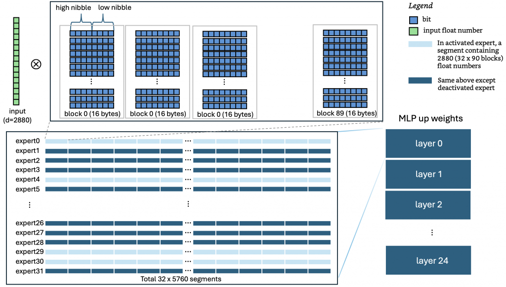
The gpt-oss models use an MXFP4 quantization for MLP layer weights. In this format, each weight is stored using just 4 bits, with an additional block-level scale factor in U8 format, the rest of the parameters are stored in BF16 (bfloat16). Find more in the Hugging Face model card. This 4-bit representation reduces the memory footprint and speed up computation during inference. Because CPU doesn’t natively support such data types, compute-heavy components like attention and the MLP projections must be executed using IEEE 754 single-precision floats. That means we need to process the 4-bit weights into floats before doing math. How efficiently we do with this has a big impact on overall performance.

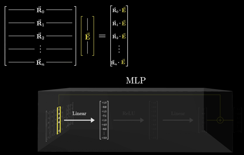
Let’s walk through what MXFP4 world looks like in practice, using the MLP up-projection of gpt-oss-20b as example. In decode phase, the model goes through 24 layers, each layer contains 32 experts. Within each layer, the input tensor is first normalized by RMSNorm to produce a 2880-dim input vector. Then, the layer selects 4 best experts to perform the up projection, and output a 5760-dim vector. Each expert’s weight tensor has a shape of [5760, 2880], it means a 2880-dim input vector gets multiplied by a 5760×2880 matrix. 3Blue1Brown visualizes the process of multiplying a long vector E (2880-dim) by a matrix R ([5760×2880]).

Now, here’s where the engineering gets interesting. On GPU, people rely on cuBLAS, CUTLASS, or custom CUDA programing to compute. On CPUs, the same principles apply — we exploit thread-level and instruction-level parallelism, maximize pipeline utilization, and avoid memory stalls. MXFP4 packs two 4-bit weights per byte in little-endian order: one in the high nibble, one in the low nibble. SIMD instructions like mm_shuffle_epi8 in cpp can unpack and extract nibbles across multiple bytes in parallel, storing them into the CPU’s vector unit. Each nibble serves as an index into below lookup table. The look-up values are then multiplied in parallel by the block-level scale factors, interleaved (high and low), and combined with the input vector using FMA (Fused Multiply–Add) instructions for parallel dot-product accumulation. Each stage of this pipeline benefits from instruction-level parallelism.

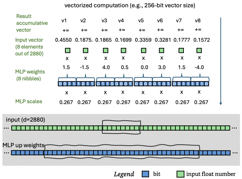
In this project, Java’s Project Panama Vector API is adopted. This leads to efficient MXFP4 computation in Java. When working together with multi-threaded parallelism, we can speed up the entire computation-intensive process.

5. Performance optimization

Out of the box, on an AWS m5.4xlarge instance (8 physical cores, 16 vCPUs), the baseline performance of the original PyTorch implementation during decode phase is only 0.04 tokens per second. A direct Java port of the PyTorch code won’t perform well even though the JVM and JIT compiler are powerful. So, I implemented several key optimizations. It turns out that on the same EC2 instance, it can get a speedup of ~7 tokens/sec for decode and ~10 tokens/sec for prefill.

5.1 Matrix Multiplication (matmul) Optimization

In essence, an LLM consists of two main components: the executable program and the model weights. The program is basically a series of linear algebra operators, most of which boil down to matrix multiplications.

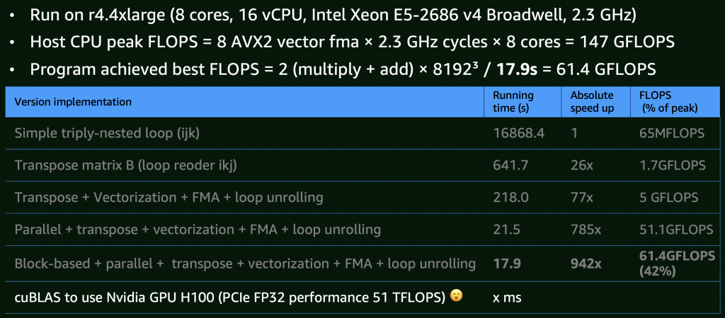
To articulate the optimization, I benchmarked 8K×8K matrix multiplications on an m4.4xlarge EC2 instance (8 physical cores, 16 vCPUs). The incremental results are:

– Baseline: A simple triple-nested loop (O(n3)) implementation, this version performed poorly.

– CPU Cache Optimization: To improve CPU cache spatial locality, by transposing matrices or storing model parameters sequentially in memory, performance improved by 26x.

– Vectorization: Using Java Project Panama’s Vector API to issue CPU SIMD instructions with 4x loop unrolling to reduce instruction dependencies, accelerated by 77x.

– Multithreading: Utilizing all CPU cores, 785x of the baseline.

– Block/Tile Computation: Finally, applying block-based matrix multiplication to maximize CPU cache hits achieved a 942x speedup. At this stage, the implementation reached about 42% of the theoretical 147 GFLOPS limit of this CPU. Given that memory stalls can still interrupt the pipeline, optimization pauses here (Interestingly, even Intel’s MKL library doesn’t fully saturate CPU).

For comparison, a GPU such as NVIDIA H100, even without using Tensor Cores, just Cuda Core, it can reaches ~51 TFLOPS in FP32 in theory — about three orders of magnitude faster than the CPU implementation. This clearly illustrates why GPUs are widely adopted in large-scale parallel computation, while CPUs are better for general-purpose workloads.

For reference, you can check out the actual implementation in gpt-oss.java here.

5.2 Parallel computation

To fully utilize CPU, parallelization is also applied to other stages including the scaled dot-product attention in GQA and the execution of the 4 experts in the MLP layer.

5.3 Memory mapping

The project uses Java’s Foreign Memory API to load MLP weights via memory mapping (mmap). This allows the model to run in as little as 16 GB of memory. The larger RAM, the page cache can hold more of the MLP weights, minimizing disk I/O in critical inference path..

5.4 Reducing unnecessary memory allocation and copying

During the up and down projections in the MLP layer, the weights are memory-mapped. Since Java’s SIMD Vector API can load data directly from mapped memory segment to CPU vector registers, this avoids intermediate indirectional JVM-level memory copies.

In addition, the code preallocates many intermediate buffers for reuse during inference. All subsequent operations read and write in place. Although the JVM’s GC is powerful, adopting a GC-less programming style wherever possible helps avoid somewhat runtime overhead.

5.5 Fused Operations

Many computations can be combined together allowing for operation fusion. However, to maintain code readability and maintainability, the current implementation only applies this selectively.

5.6 KV Caching

Almost all modern LLM inference engines use KV caching. This project takes a simpler approach: the KV cache is preallocated based on the maximum token length. Thanks to Grouped Query Attention (GQA), memory usage is significantly reduced compared to classic Multi-Head Attention (MHA)

5.7 Performance Results

– MacOS (Apple M3 Pro): Decode speed — 8.7 tokens/sec, Prefill speed — 11.8 tokens/sec

– AWS EC2 m5.4xlarge (8 cores, 16 vCPUs): Decode speed — 6.8 tokens/sec, Prefill speed — 10 tokens/sec

This represents a dramatic improvement over the original educational PyTorch implementation (0.04 tokens/sec) and outperforms Hugging Face Transformers (~3.4 tokens/sec).

However, it still trails behind llama.cpp running the MXFP4 GGUF v3 model, which reaches 16.6 tokens/sec. That difference mainly comes from llama.cpp’s lower-level SIMD usage, more refined thread scheduling, deeper kernel optimizations, and of course, C++’s performance advantage over Java.

More detailed performance data can be found here.

6. Implementation Summary

This project is valuable in learning. With just about 1,000 lines of code, it reimplemented an MoE-based LLM from scratch. The process of porting deepens the understanding of PyTorch and its great abstraction. With building blocks functions/modules that fit together like LEGO, PyTorch makes model development easy, that in turn, makes the Java port much smoother.

Performance perspective, the results are quite solid. Of course, for a better user experience and higher performance, dedicated edge-device single-host inference engines such as Ollama and LM Studio are still preferred. LLM inference has become an engineering hotspot, and its performance depends on low-level optimizations. Industrial frameworks like vLLM, SGL, TensorRT-LLM, and ONNX Runtime represent the state of the art in high-performance inference.

Java performance continues to advance: Project Leyden reduces startup latency, Lilliput optimizes object layout, Loom introduces virtual threads, Panama bridges Java and native code, and Valhalla enables more compact object representations. Also, with improved ZGC and AOT (GraalVM) support, these improvements are closing the performance gap between Java and lower-level languages. In my earlier llama2.c -> llama2.java porting project, I verified that Java could achieve about 95% of the performance of an O3-optimized C version. This demonstrates that Java can run fast — as long as performance hotspots are properly identified and optimized.